Posts

Showing posts with the label Physics

Estimation of the Rydberg Constant

Image
The aim of this experiment is to make an estimation of the Rydberg constant based on measurements of the wavelengths of visible lines on the atomic spectrum of hydrogen, also known as the Balmer series. In Part A of the experiment, a linear model is derived that represents the change in measured wavelength given expected wavelength values of the atomic spectra of mercury. This is just used as an initial comparison to ensure the spectrometer is calibrated. Part B of the experiment is intended to obtain a linear function that represents the change in 1/wavelength given 1/n2. The slope of this linear model is taken to determine an estimation of the Rydberg constant. The variables being used in the experiment are as follows: λ1 = A single column data table containing the measured wavelengths of each visible line on the mercury spectrum. λ2 = A single column data table containing the measured wavelengths of each visible line on the balmer series of the hydrogen spectrum. λa1 = A s

How to Measure the Horizontal Component of Earth's Magnetic Field

Image
The aim of this experiment is to find the magnitude of the magnetic field produced by a current carrying circular coil. Using the experimental values obtained from the following experiments, it is possible to estimate the horizontal component of the earth’s magnetic field. In Part A of the experiment, a function is derived that represents the tangent of the change in the angle shown on a compass positioned in the center of a circular coil in terms of the number of turns in the coil. Part B of the experiment is intended to derive a function that represents the tangent of the change in angle of a compass needle positioned in the center of a circular coil in terms of the input current. The variables being used in each experiment are as follows: Θ = The number of degrees the compass needle is displaced when the coil is charged. i = current in Amperes. N = the number of turns of the coil. Bh = estimation of the horizontal component of the earth’s magnetic field Be1 = An estimati

How to Determine the Velocity of Sound

Image
The aim of this experiment is to determine the Velocity of sound in air by measuring the resonant frequency of air columns of variable length. The variables being used in the experiment are as follows: L = Length of air column (meters) f = resonant frequency (Hertz) c = Velocity of sound (meters/second) t = air temperature (Celsius) x = 1/f, the reciprocal of the measured resonant frequency (period) (seconds) y = Length of the air column (meters) m = slope of the linear regression (meters/second) e = y intercept Experimental Method A speaker and oscillator was used to produce and record standing waves within a plastic cylinder, closed at one end, in order to determine the velocity of sound in air. The oscillator was first adjusted to a reasonable volume at 250 Hz so that the experimenters could hear the tone produced by the speaker. The cylinder was also emptied of any liquid that may have been inside. Given the accepted value of the velocity of sound in air at 0֯

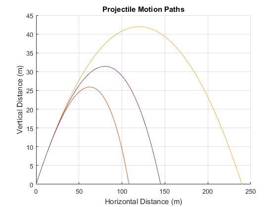
Projectile Motion Paths in MatLab

Image
The following is a MATLAB script which produces the projectile paths of a spherical object, such as a cannonball, given  radius (r), mass (m), initial velocity (v), and angle above the horizontal (theta) . By changing the experimental variables mentioned above, and others attributed to the environment, such as the  density of air (rho) ,  gravity (g)  and the  drag coefficient (C)  the various effects can be visualised in the graph this script outputs.  ifr=1; C=0; C1 = 0.5; theta=35;    v = 50;        g= 9.80;     dt = 0.0001;  i = 1; max_iters = 1000000; x(1) = 0; y(1) = 0; x1(1) = 0; y1(1) = 0; t0 = 0; while ifr<=2     r=0.036*ifr;     m=0.145*ifr^3;     rho=1.2;          A=pi*r^2; A1=pi*r^2;     D=rho*C*A/2; D1=rho*C1*A1/2;          vx =v*cosd(theta); vx1 =v*cosd(theta);     vy =v*sind(theta); vy1 =v*sind(theta);       while y(i) >= 0 && i < max_iters           ay=-g; ay1=-g-(D1/m)*(vx1^2+vy1^2)^0.5*vy1;