Estimation of the Rydberg Constant
The aim of this experiment is to make an estimation of the Rydberg constant based on measurements of the wavelengths of visible lines on the atomic spectrum of hydrogen, also known as the Balmer series.
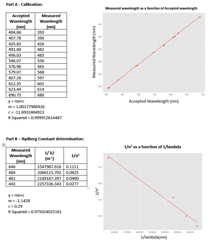
In Part A of the experiment, a linear model is derived that represents the change in measured wavelength given expected wavelength values of the atomic spectra of mercury. This is just used as an initial comparison to ensure the spectrometer is calibrated.
Part B of the experiment is intended to obtain a linear function that represents the change in 1/wavelength given 1/n2. The slope of this linear model is taken to determine an estimation of the Rydberg constant.
The variables being used in the experiment are as follows:
λ1 = A single column data table containing the measured wavelengths of each visible line on the mercury spectrum.
λ2 = A single column data table containing the measured wavelengths of each visible line on the balmer series of the hydrogen spectrum.
λa1 = A single column data table containing the accepted wavelengths of each visible line on the mercury spectrum.
λa2 = A single column data table containing the accepted wavelengths of each visible line on the balmer series of the hydrogen spectrum.
ɛ02 = 8.85418782 × 10⁻¹² (The permittivity of free space)
M = mass of electron (9.10938356 × 10⁻³¹ kilograms)
e = charge of an electron (1.60217662 × 10⁻¹⁹ coulombs)
V = the speed of light (299,792,458 meters/second)
h = the Planck constant
Equipment:
1 x Bellingham and Stanley direct reading wavelength spectrometer
1 x Hydrogen spectral discharge tube with EHT power supply
1 x Mercury vapour lamp with power supply
Experimental Method
Before measuring the wavelength of the spectral lines of the balmer series of hydrogen for the main part of the experiment, the spectrometer needed to be calibrated to minimise error in the results. In order to ensure it was calibrated, a table of data representing the accepted wavelengths of visible light emitted from the mercury spectrum was used.
By taking measurements of the mercury lamp spectral wavelengths, and comparing them with this set of known mercury spectral data, an R squared value can be determined with an analysis of variance to determine how closely the measured results fit with the known values.
Once you can be sure the spectrometer is calibrated and the measured data aligns with known values, the balmer series can be examined and wavelengths can be measured for the visible light given off by the hydrogen spectrum.
Part A – Calibration of spectrometer:
Part B – Determining Rydbergs constant:
Results

Data Analysis
The data for Part A was stored in a data array consisting of two columns, x1 and y1. x1 is a list of the values of accepted wavelengths of visible lines in the mercury spectrum used in Part A of the experiment. y1 is a list of the measured wavelength results from part A
The data for Part B was stored in a data array consisting of two columns, x2 and y2. x2 is a list of the values of 1/λ2 used in Part B of the experiment. Y2 is a list of the 1/n2 results from part B.
Both sets of data were linear and could be represented by the standard linear equation y = mx+c. The ANOVA (analysis of variance) method was used to determine several useful pieces of information in terms of each regression model. The following set of equations were used to obtain the slope for each part of the experiment.
meanx = sum(x)/len(x)
meany = sum(y)/len(y)
meanxx = sum(x*x)/len(x)
meanx = sum(x*y)/len(y)
m = ((meanx*meany)-meanxy)/((meanx**2)-meanxx)
c = meany-m*meanx
The following equation was used to determine a theoretical value for the Rydberg constant:
R = (1/ɛ02)*((M*e4)/(8*V*h3))
= (1/ɛ02)*((M*e**4)/(8*V*h**3))
= 10973731.5427347
Experimental Discussion
There was a difference between the two calculations of the Rydberg constant by about 450,000, which is close to 4.5%. This could be attributable to many factors, for example, the placement of the lamp or spectral discharge tube need to be precise and aligned correctly so that spectral lines can be seen properly, especially as you approach invisible light. It is possible that while calibrating the spectrometer, the lines were made too think or too thin resulting in inaccurate measurements at the centre of each line.
Also, there were only 4 visible lines to measure in the balmer series, so measuring ultraviolet or infrared lines would allow for more data, increasing the likelihood of a tighter linear model, along with a better representation of the rydberg constant.
Conclusion
The coefficient of determination of the Part A of the experiment was 0.99991 showing that the data matched the linear model with a high level of accuracy and that the spectrometer was properly calibrated.
The coefficient of determination of Part B of the experiment was insufficient at 0.975, implying that although the data was highly correlated, using the function from part B would not yield accurate estimations of the Rydberg constant, an R squared value of 0.99 or greater would be preferred, especially when dealing with objects in the atomic scale because even a small amount of error can translate to a relatively huge difference.
In Part A of the experiment, a linear model is derived that represents the change in measured wavelength given expected wavelength values of the atomic spectra of mercury. This is just used as an initial comparison to ensure the spectrometer is calibrated.
Part B of the experiment is intended to obtain a linear function that represents the change in 1/wavelength given 1/n2. The slope of this linear model is taken to determine an estimation of the Rydberg constant.
The variables being used in the experiment are as follows:
λ1 = A single column data table containing the measured wavelengths of each visible line on the mercury spectrum.
λ2 = A single column data table containing the measured wavelengths of each visible line on the balmer series of the hydrogen spectrum.
λa1 = A single column data table containing the accepted wavelengths of each visible line on the mercury spectrum.
λa2 = A single column data table containing the accepted wavelengths of each visible line on the balmer series of the hydrogen spectrum.
ɛ02 = 8.85418782 × 10⁻¹² (The permittivity of free space)
M = mass of electron (9.10938356 × 10⁻³¹ kilograms)
e = charge of an electron (1.60217662 × 10⁻¹⁹ coulombs)
V = the speed of light (299,792,458 meters/second)
h = the Planck constant
Equipment:
1 x Bellingham and Stanley direct reading wavelength spectrometer
1 x Hydrogen spectral discharge tube with EHT power supply
1 x Mercury vapour lamp with power supply
Experimental Method
Before measuring the wavelength of the spectral lines of the balmer series of hydrogen for the main part of the experiment, the spectrometer needed to be calibrated to minimise error in the results. In order to ensure it was calibrated, a table of data representing the accepted wavelengths of visible light emitted from the mercury spectrum was used.
By taking measurements of the mercury lamp spectral wavelengths, and comparing them with this set of known mercury spectral data, an R squared value can be determined with an analysis of variance to determine how closely the measured results fit with the known values.
Once you can be sure the spectrometer is calibrated and the measured data aligns with known values, the balmer series can be examined and wavelengths can be measured for the visible light given off by the hydrogen spectrum.
Part A – Calibration of spectrometer:
- The mercury lamp was placed infront of the spectrometer entrance slit by hand so that it was aligned as evenly and close to it as possible.
- The spectrum was viewed through the telescope and the drum adjusted so that one of the visible lines could be seen comfortably. (the slit wedge was widened or limited if the line being viewed needed height adjustments to be easily seen. The screw around the slit wedge was adjusted when width adjustments were required.)
- A measurement of the wavelength for the current line being viewed was taken in nanometers and recorded next to the accepted values.
- The drum was adjusted to find other lines in the mercury spectrum and step 3 was repeated for each of the supplied values of accepted wavelengths to make λ1.
- Linear regression using the ANOVA method was performed on the table of accepted vs measure wavelengths and an R squared value was determined to measure the tightness of fit to confirm the spectrometer was outputting the correct information.
Part B – Determining Rydbergs constant:
- The mercury lamp was removed from the entrance slit, replaced with the hydrogen spectral discharge tube, and the EHT power supply was turned on.
- The 4 visible lines in this spectrum were much fainter than the lines in the mercury spectrum and so, much like during calibration, some slight adjustments were made until the spectral lines were comfortably visible.
- Starting at the red line, a measurement of the wavelength of each visible line was recorded to make λ2.
- 1/ λ2 was determined and each value of this set of data was compared against 1/n2 , to obtain a linear set of data.
- ANOVA was performed on 1/ λ2 versus 1/n2 to obtain a slope which represents the Rydberg constant.
Results
Data Analysis
The data for Part A was stored in a data array consisting of two columns, x1 and y1. x1 is a list of the values of accepted wavelengths of visible lines in the mercury spectrum used in Part A of the experiment. y1 is a list of the measured wavelength results from part A
The data for Part B was stored in a data array consisting of two columns, x2 and y2. x2 is a list of the values of 1/λ2 used in Part B of the experiment. Y2 is a list of the 1/n2 results from part B.
Both sets of data were linear and could be represented by the standard linear equation y = mx+c. The ANOVA (analysis of variance) method was used to determine several useful pieces of information in terms of each regression model. The following set of equations were used to obtain the slope for each part of the experiment.
meanx = sum(x)/len(x)
meany = sum(y)/len(y)
meanxx = sum(x*x)/len(x)
meanx = sum(x*y)/len(y)
m = ((meanx*meany)-meanxy)/((meanx**2)-meanxx)
c = meany-m*meanx
The following equation was used to determine a theoretical value for the Rydberg constant:
R = (1/ɛ02)*((M*e4)/(8*V*h3))
= (1/ɛ02)*((M*e**4)/(8*V*h**3))
= 10973731.5427347
Experimental Discussion
There was a difference between the two calculations of the Rydberg constant by about 450,000, which is close to 4.5%. This could be attributable to many factors, for example, the placement of the lamp or spectral discharge tube need to be precise and aligned correctly so that spectral lines can be seen properly, especially as you approach invisible light. It is possible that while calibrating the spectrometer, the lines were made too think or too thin resulting in inaccurate measurements at the centre of each line.
Also, there were only 4 visible lines to measure in the balmer series, so measuring ultraviolet or infrared lines would allow for more data, increasing the likelihood of a tighter linear model, along with a better representation of the rydberg constant.
Conclusion
The coefficient of determination of the Part A of the experiment was 0.99991 showing that the data matched the linear model with a high level of accuracy and that the spectrometer was properly calibrated.
The coefficient of determination of Part B of the experiment was insufficient at 0.975, implying that although the data was highly correlated, using the function from part B would not yield accurate estimations of the Rydberg constant, an R squared value of 0.99 or greater would be preferred, especially when dealing with objects in the atomic scale because even a small amount of error can translate to a relatively huge difference.
Comments
Post a Comment